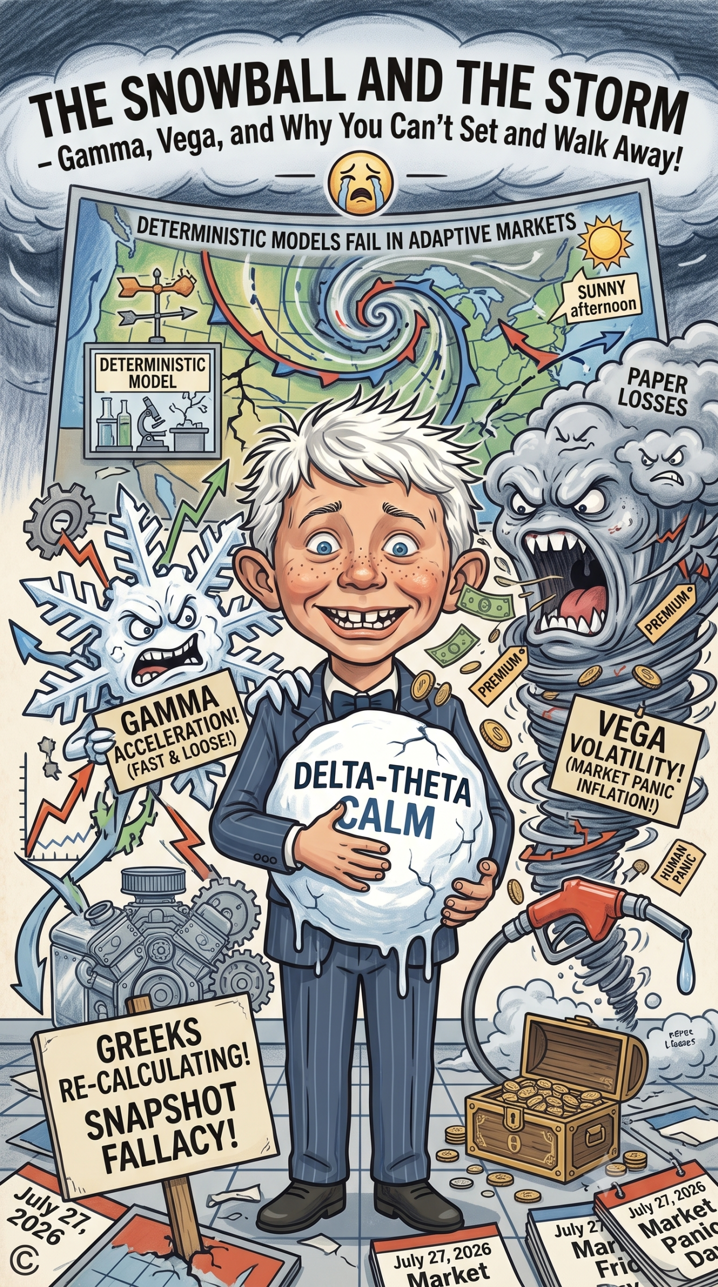
Gamma, Vega, and Why Deterministic Models Fail in Adaptive Markets
In Part 1, we established our baseline time-decay engine using Delta and Theta. We mapped out our portfolio, calculated our Delta-to-Theta ratio, and examined why treating financial markets like static physical structures is a dangerous fallacy.
If options trading ended with Delta and Theta, you could simply set up your positions, collect daily time decay, and walk away. But as every experienced options seller knows, the market is not a peaceful laboratory.
When human panic sets in, the math changes.
While Delta and Theta tell you how your portfolio looks on a calm, sunlit afternoon, Gamma and Vega are the storm indicators. They measure how fast your risk accelerates when market participants stop acting rationally and start running for the exits.
The Fallacy of the Bell Curve: Fat Tails and Human Madness
Highly analytical minds—software developers, data scientists, accountants, engineers, and quants—bring unmatched strengths to options trading. They excel at structural mechanics, risk modeling, and systematic discipline.
The trap isn’t intelligence or technical skill; it’s methodology transfer. Quantitative training often conditions us to treat problems as deterministic systems governed by neat probability distributions. Standard options pricing models rely on this exact same assumption: that stock returns follow a log-normal bell curve.
Under a pure bell curve model:
- A 3-standard-deviation market move should happen about once every few years.
- A 5-standard-deviation crash should happen once every few thousand years.
- A 10-standard-deviation event shouldn’t happen in the lifespan of the universe.
Yet, in real financial markets, 5- and 10-standard-deviation crashes happen every few years.
Standard Normal Distribution (The Model's Assumption)
               /\
              /  \
             /    \
  __________/______\__________

Real Market Distribution (Fat Tails / Human Reality)
              _/\_
             /    \   <-- High Peak (More sideways days)
            /      \
  _________/________\_________  <-- Fat Tails (Frequent Extreme Panics)
Why does the math fail so spectacularly? Because physical probability models assume independent events. If a blue marble is drawn from an urn, it doesn’t make the next marble terrified.
In financial markets, events are deeply dependent. When one institutional fund is forced to liquidate, its selling drops the price, which triggers automated stop-losses for other funds, which causes retail traders to panic-sell on their phone apps.
Trying to fit complex human behavior into a static bell curve isn’t just inaccurate—it’s catastrophic for anyone taking on unmanaged risk.
Gamma (Γ): The Accelerator Pedal
If Delta is your speedometer, Gamma is the accelerator pedal.
Mathematically, Gamma measures how fast your Delta changes for every $1.00 move in the underlying stock:
Gamma = Change in Delta / Change in Stock Price
When you sell short options (short puts or short calls), you are short Gamma.
The Snowball Effect
Being short Gamma means that as the market moves against you, your directional exposure automatically expands in the worst possible direction:
- You sell a -20 Delta put option (mildly bullish exposure).
- The stock drops suddenly by $5.00.
- Because of Gamma, that option’s Delta doesn’t stay at -20. It expands to -45 Delta.
- Now, every subsequent drop in the stock hurts your account more than twice as fast as the initial drop.
This is why Gamma is known as the “snowball metric.” On calm days, Gamma sits quietly in the background. But during a sharp selloff, short Gamma acts like a magnet pulling your portfolio toward maximum pain.
Vega (ν): The Pricing of Human Fear
Vega measures how sensitive an option’s theoretical value is to changes in Implied Volatility:
Vega = Change in Option Value / 1% Change in Implied Volatility
Implied Volatility is not a measure of historical price movement. It is a forward-looking calculation derived directly from current option prices. When market participants get nervous and rush to buy downside protection, demand for options skyrockets. Market makers respond by marking up option prices across the board.
In plain terms: Implied Volatility is the market’s fear index.
Looking Back at Our Portfolio Case Study
Recall our combined portfolio metrics from Part 1:
| Portfolio Level | Total Net Liq | Aggregate Delta | Aggregate Theta | Aggregate Vega |
| COMBINED TOTALS | $137,750.00 | +119 | +431 | -1,968 |
Notice that our portfolio has a Vega of -1,968. This means our portfolio is heavily short volatility.
- If Implied Volatility drops by 1 percentage point, our account theoretically gains +$1,968.00.
- If Implied Volatility spikes by 3 percentage points during a sudden market panic, our account takes an immediate paper loss of approximately -$5,904.00 (-1,968 × 3), even if underlying stock prices haven’t moved much yet!
How the Greeks Behave Under Stress
| Market Scenario | Delta Impact | Gamma Effect | Vega Effect | Portfolio Result |
| Sideways Drift | Stable (+119) | Minimal | Shrinking (Theta wins) | Daily Cash Accrual (+$431/day) |
| Mild 2% Pullback | Increases slightly | Mild acceleration | Slight IV expansion | Minor paper drawdown; easily managed |
| Sharp 5%+ Crash | Expands rapidly | Snowballs against position | Spikes massively (Vega inflated) | Heavy paper losses; Buying Power expands |
The AI Fallacy: When “Self-Adjusting” Machines Are Left Unsupervised
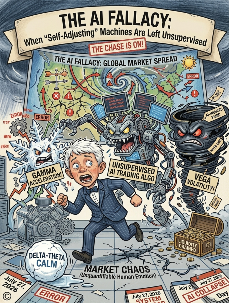
A popular myth in modern trading is that the rise of adaptive, self-adjusting AI will finally stabilize markets. Modern algorithmic models are no longer just rigid scripts—they use deep reinforcement learning to adjust parameters in real time, detect system anomalies, and execute automated subroutines when risk limits are breached.
The reality is the exact opposite when machines are left unsupervised.
Self-repairing code sounds great on an engineering blueprint, but in financial markets, an AI’s idea of a “repair” often causes the crash. When an adaptive model encounters an unprecedented wave of human panic, it doesn’t possess common sense or macro-context. Its neural networks re-calculate risk on the fly and attempt to self-correct by aggressively shorting momentum, liquidating collateral, or pulling quotes entirely to protect its own capital.
The machine successfully “repairs” its own risk metrics—by burning down the rest of the market’s liquidity.
No matter how advanced or self-correcting a trading model claims to be, it still requires constant human handholding. A human trader can look at a geopolitical event or a sudden liquidity void and say, “Wait, the math says sell, but the room is on fire—stand down.” An unsupervised AI just executes the math faster, turning localized adjustments into systemic feedback loops.
History provides clear examples of what happens when unsupervised algorithms collide with unexpected human behavior:
1. The “Yen Carry Trade” Volatility Surge (August 2024)
- The Trigger: The Bank of Japan raised interest rates, strengthening the Yen and triggering the rapid unwind of leveraged cross-border carry trade positions.
- The Algorithmic Loop: Hundreds of automated volatility-targeting strategies and algorithmic CTAs read market risk through real-time volatility meters. As pre-market liquidity thinned, the algorithms misinterpreted the widening spreads as systemic danger. They automatically dumped equity positions worldwide, driving Japan’s TOPIX and Nikkei down 12% in a single trading session—as detailed by the Bank for International Settlements Report, this was the market’s worst single-day drop since Black Monday in 1987—and triggering a global market slide before human managers could step in.
2. The 2010 “Flash Crash” ($1 Trillion Automated Cascade)
- The Trigger: According to the official CFTC & SEC Joint Report, an institutional mutual fund entered an automated execution algorithm to sell 75,000 E-mini S&P 500 futures contracts (worth roughly $4.1 billion) at a targeted 9% participation rate without price or time controls.
- The Algorithmic Loop: High-Frequency Trading (HFT) algorithms began buying and dumping the contracts back and forth in an automated “hot potato” effect. When risk thresholds were breached, the HFT algorithms simultaneously withdrew all buy quotes from the order books. Without buying support, the Dow Jones plunged nearly 1,000 points (about 9%) in minutes, erasing nearly $1 trillion in market value before recovering once human intervention stepped in.
3. Black Monday (October 19, 1987)
- The Trigger: Rising interest rates and growing international trade deficits caused underlying market jitteriness.
- The Algorithmic Loop: Wall Street had widely adopted “Portfolio Insurance”—the earliest primitive form of algorithmic trading designed to protect against downside risk by automatically shorting futures as stock prices fell. As the market opened down, computer models triggered automated sell orders simultaneously. That selling pushed prices lower, which triggered the next tier of computer sell orders. As documented by the Federal Reserve’s Historical Records, the feedback loop resulted in the Dow plummeting 22.6% in a single day—the largest single-day percentage decline in stock market history.
4. The “Quant Quake” (August 2007)
- The Trigger: Early cracks in subprime mortgage debt forced several multi-strategy funds to liquidate positions, shifting quantitative factor exposures.
- The Algorithmic Loop: Quantitative equity hedge funds relied on mathematical models that assumed historical factor correlations were permanent. When initial liquidations caused minor paper losses, risk-management algorithms across competing funds misread the moves as factor breakdowns. The computers automatically began liquidating long positions and shorting losing positions across the board. As documented by research from the National Bureau of Economic Research (NBER), because dozens of unsupervised funds ran similar quantitative models, the algorithms wiped out billions of dollars in equity across high-quality, uncorrelated stocks in just 72 hours.
[ Sudden Macro Trigger or Unexpected Order ]
                     ↓
[ Unsupervised AI Misinterprets Volatility as Structural Breakdown ]
                     ↓
[ Automated "Self-Repair" Pulls Liquidity & Dumps Collateral ]
                     ↓
[ Order Book Collapses → Spikes Volatility → Triggers Next Layer of Models ]
                     ↓
[ Automated Flash Crash ]
The fundamental flaw in trading algorithms is that they lack human context. They operate on historical probabilities. When human fear causes a sudden shift in market behavior, those mathematical probabilities break down, and the unsupervised algorithms amplify human panic instead of solving it.
The Casino vs. The Bridge: Managing Probabilities, Not Trajectories
This brings us to the core realization that separates amateur traders from seasoned professionals:
We cannot predict human behavior, but we can price human emotion.
When you sell an option, you are not predicting where a stock will go. You are acting as an insurance underwriter. You are identifying moments when market participants are overpaying for protection out of fear, establishing wide statistical safety margins, and collecting the premium.
Where analytical minds frequently blow up is mistaking high probability for absolute certainty.
An engineer designing a bridge targets a structural failure probability close to zero. An options trader operating at an 84% probability of success must accept that 16% of trades will lose.
If you size your trade positions under the assumption that an 84% probability is a “sure thing,” a single 3-standard-deviation storm will wipe out months of Theta collection in a single afternoon.
What’s Next?
Understanding Gamma, Vega, and algorithmic feedback loops gives us respect for the market’s tail risk—but understanding risk is only half the battle. Now we have to analyze our full health dashboard and put execution rules into practice.
In Part 3: Your Portfolio’s Health Dashboard, we will unlock the remaining key metrics on our trading platform:
- Theta-to-Net-Liq (The Daily Yield): How to calculate your account’s daily cash generation rate and stay in the optimal yield sweet spot.
- Theta-to-Vega (The Rent-to-Storm Shield): How to measure whether your daily income is strong enough to cushion a sudden volatility spike.
- The Realized vs. Theoretical Theta Gap: Why your daily Theta metric isn’t a guaranteed daily paycheck, and how to manage the gap between theoretical decay and realized cash flow.
References & Further Reading
- Lo, Andrew W. and Mueller, Mark T. (2010). “Physics Envy: An Alternate Perspective of Economic Behavior.”MIT Laboratory for Financial Engineering. (Paper PDF)
- Bookstaber, Rick (2010). “Physics Envy in Finance.” Rick Bookstaber’s Blog. (Blog Post)
- Bank for International Settlements (2024). “The market turbulence and carry trade unwind of August 2024.” (BIS Report PDF)
- Joint CFTC-SEC Advisory Committee (2010). “Findings Regarding the Market Events of May 6, 2010.”(CFTC/SEC Report PDF)
- Federal Reserve History. “Stock Market Crash of 1987 (Black Monday).” (Fed Reserve History)
- Khandani, Amir E. and Lo, Andrew W. (2007/2008). “What Happened To The Quants In August 2007?” National Bureau of Economic Research. (NBER Paper PDF)
- tastylive Insights (2023). “How to Put Delta and Theta to Work.” (tastylive Article)
- Natenberg, Sheldon. Option Volatility and Pricing: Advanced Trading Strategies and Techniques. McGraw-Hill.
- Taleb, Nassim Nicholas (2007). The Black Swan: The Impact of the Highly Improbable. Random House.