

I took a gamble on this trade and it was a complete bust. An expensive lesson.
🎓 The $1,000 Seminar: Why Peak Volatility is a Calendar Killer – HIGH NOON TRADER
Periods of elevated volatility often create opportunities in the options market that aren’t available during calmer conditions. With geopolitical tensions rising, gas spiking 30% overnight, and volatility spiking, I recently entered a double diagonal options trade in E-mini S&P 500 futures (ES) designed to take advantage of expensive short-term volatility and a steep volatility term structure.
Rather than betting on a strong directional move, this trade focuses on harvesting time decay and exploiting volatility differences across expirations.
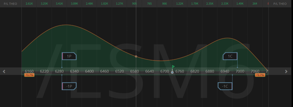
📊 Market Snapshot at Entry
At the time the trade was entered, the market environment looked like this:
| Metric | Value |
|---|---|
| Underlying | ES ≈ 6991 |
| Key resistance | 7000 |
| VIX | ≈ 29 |
| Front IVx (15D) | 44.9% |
| Back IVx (~40D) | 38.8% |
This environment is notable because near-term implied volatility was significantly higher than longer-dated volatility, creating an opportunity to sell expensive premium in the short term while owning cheaper volatility further out in time.
🧩 Trade Structure

The position is a 15-day / 39-day double diagonal, constructed with the following legs:
| Leg | Expiration | Strike | Action |
|---|---|---|---|
| Put | Mar 23 (15D) | 6250 | Sell |
| Call | Mar 23 (15D) | 6930 | Sell |
| Put | Apr 17 (39D) | 6250 | Buy |
| Call | Apr 17 (39D) | 6950 | Buy |
Position Metrics
| Metric | Value |
|---|---|
| Total Debit | $5,225 |
| Delta | ~0.02 |
| Theta | +141.88 |
The trade begins nearly market neutral, meaning it does not rely heavily on predicting the exact direction of the S&P 500. Instead, it focuses primarily on time decay and volatility behavior.
🌪️ The Volatility Edge
The main edge in this setup comes from the term structure of volatility.
| Expiration | Implied Volatility |
|---|---|
| ~15 Days | 44.9% |
| ~40 Days | 38.8% |
This creates a spread of roughly 6 volatility points between short-term and longer-dated options.
In practical terms, the trade is:
- 🔻 Selling expensive short-term volatility
- 🔺 Buying cheaper longer-dated volatility
If volatility normalizes or declines, the front-month options should decay faster than the back-month options, which benefits the structure.
This type of setup is particularly attractive during periods when markets are pricing in near-term uncertainty or panic.
🌍 Market Context
Market conditions leading into the trade also supported the setup.
The S&P 500 had recently experienced a roughly 2% decline, and further short-term weakness remained possible. Moderate downside or sideways movement would move price closer to the center of the trade’s profit zone.
Additionally, the 7000 level in ES futures had been acting as a key psychological resistance level. Placing the short call just below this level (6930) allows the trade to collect premium in an area where rallies have recently stalled.
This positioning creates a favorable balance:
- limited directional exposure
- strong premium collection
- room for normal market fluctuations
⚠️ Hidden Volatility: Crash Skew
Another important component of the trade is downside crash skew.
In equity index options, out-of-the-money puts usually trade at higher implied volatility than calls. This happens because institutions frequently buy puts as portfolio insurance.
Even with the VIX already near 29, the options market still showed strong demand for downside protection.
In other words:
The market was still pricing in the possibility of a sharp downside event.
This creates an opportunity because short-dated options contain fear-driven volatility premiums.
By selling short-term options while maintaining distance from the downside strike (6250), the trade collects some of this inflated premium without sitting directly in the crash zone.
📐 Position Profile
At entry, the Greeks describe a position designed to benefit primarily from time decay.
| Greek | Value | Interpretation |
|---|---|---|
| Delta | ~0.02 | Nearly market neutral |
| Theta | +141.88 | Strong positive time decay |
| Vega | Positive | Benefits from volatility normalization |
This means the position benefits most from:
- ⏳ Time passing
- 🌡️ Short-term volatility declining
- 📊 Moderate price stability
✅ What Would Help the Trade
The ideal outcome for this structure involves limited directional movement combined with volatility cooling off.
| Market Behavior | Effect |
|---|---|
| Sideways price action | Best outcome |
| Mild pullback | Positive |
| Volatility decline | Strongly positive |
| Price near short strikes at expiration | Maximum time decay |
A moderate move toward 6800–6900 would bring the underlying closer to the center of the trade’s profit profile, accelerating decay in the short options.
⚡ Main Risk
Like most premium-selling structures, the biggest risk comes from large directional moves.
| Scenario | Risk |
|---|---|
| Rally above 7000 | Short call becomes pressured |
| Strong relief rally | Directional move + volatility collapse |
| Large trending move | Short-dated gamma exposure |
If the market were to break strongly above resistance, adjustments such as rolling short strikes higher could be considered.
🧠 Conclusion
This double diagonal is a volatility-focused strategy designed for uncertain markets.
By selling elevated short-term volatility and buying cheaper longer-dated volatility, the trade attempts to capture:
- ⏳ Time decay
- 🌪️ Volatility normalization
- 📉 Market consolidation following a volatility spike
When markets are pricing in fear — whether due to geopolitical events, macro uncertainty, or recent price shocks — strategies like this allow traders to shift the focus away from predicting direction and toward taking advantage of the volatility itself.
Leave a Reply